Predicting epileptic seizure onsets with Heart Rate Variability (HRV) features and Machine Learning (ML)
Predicting epileptic seizure onsets with Heart Rate Variability (HRV) features and Machine Learning (ML)
By Harshinee Sriram
This post was written by one of our graduate students, Harshinee Sriram, and is a report on a research project to determine the effectiveness of different machine learning (ML) models to predict epileptic seizure onsets. Harshinee’s research was inspired by one of our CIC projects: a health platform for people on the autism spectrum. Although not directly related to the project’s challenge and solution, the current report explores an important area of research that bridges the use of ML with medical practices.
The first few sections of the post detail the importance of the topic, what stages a seizure involves, and existing research done on epileptic seizure prediction. The report also offers insights into the association between epilepsy and autism, that individuals who have epilepsy are more likely to be on the autism spectrum, and vice versa.
In the sections following the literature reviews, Harshinee writes about an experiment that was done to train classical ML models to predict the onset of seizures using existing data from patients who have epilepsy. The models studied were Gradient Boosting, Adaptive Boosting, Logistic Regression, Naive Bayes, K Nearest Neighbours, Random Forest, and Support Vector Machine.
1. Introduction
Seizure is defined as a sudden, uncontrolled electrical disturbance in the brain. Seizures can cause changes in your behaviour, movements or feelings, and in levels of consciousness. A person is diagnosed with epilepsy when they have two or more seizures. According to the World Health Organization (WHO), around 50 million people worldwide have epilepsy and about 80% of them live in low- and middle-income households. Additionally, around 30% of this population experiences drug-resistant epilepsy (DRE) [Fattorusso et al 2021]. Hence, developing a cost-effective tool that helps predict when a seizure is about to occur within a reasonable amount of time is paramount. Existing state-of-the-art approaches predominantly use EEG signals and maps to predict the onset of a seizure, however, using EEG caps on a daily basis to monitor seizures is impractical. Hence, this project extends on a relatively new body-of-work that aims to predict seizures using heart rate variability (HRV) features generated from a publicly available medical dataset. We experiment with multiple HRV features and classical machine learning models to determine the best predictors for a seizure onset. Based on our results, we also draw conclusions on the importance of dataset size and quality for prediction tasks in the medical domain. We believe this work can act as a preliminary step in determining the most optimal learning architecture for this task.
2. Relationship between epilepsy and autism
There have been studies that associate epilepsy and autism (Viscidi et al 2013; Ewen et al 2019; Achkar et al 2015). These works state that children are a little more likely to have epilepsy and that children with epilepsy are a little more likely to have autism. Ewen et al (2019) have also stated that autistic women are more likely to have epilepsy than autistic men, and, in an autistic person, motor problems, language difficulties, and regression are all associated with epilepsy. When it comes to genetic commonalities, one study found that there is a significant overlap between genes linked to epilepsy and those tied to autism (Novarino et al 2013). Novarino et al (2013) also found that children who have an autistic older sibling are 70 percent more likely to have epilepsy than controls, even if they do not themselves have autism. In general, researchers have linked mutations in several genes, including SCN2A and HNRNPU to epilepsy, autism or both (Borlot et al 2019). Certain genetic conditions related to autism, such as tuberous sclerosis or Phelan-McDermid syndrome, are also associated with epilepsy (Frank et al 2021). One theory for this overlap is that both conditions (epilepsy and autism) share common biological mechanisms. Epilepsy is characterised by too much excitation in the brain, which may stem from too little inhibition.
3. Stages of a seizure
There are primarily 4 stages of a seizure episode (see figure 1), these have been described below:
- Prodrome: Some people with epilepsy say they can tell when a seizure is on the way. They may notice some signs, known as a “prodrome,” a few hours or even days before one starts. Common prodrome symptoms include: changes in mood, trouble sleeping, anxiety, problems staying focused, feeling lightheaded etc. Prodrome more pronounced in patients with generalised seizures, which are seizures that affect both sides of the brain.
Note: Prodrome more pronounced in patients with generalised seizures, which are seizures that affect both sides of the brain. In contrast, focal/partial seizures affect just one area of the brain. A person with epilepsy can experience either kind of seizure. Autism spectrum disorders (ASD) are not associated with a certain type of seizure. - Aura (pre-ictal): This pre-ictal (aura) stage happens right before a seizure starts and is a warning that it is about to happen. The symptoms come on quickly and may only last a few seconds. During this stage, common symptoms include: deja vu, vision problems, odd smells, sounds, or tastes, dizziness, numbness or “pins and needles” in parts of your body etc. Some people don’t experience this stage at all
- Ictal: During the ictal stage, intense electrical changes happen in the brain. Other people won’t notice some of the symptoms, which have been described as: feeling a gust of wind even though you’re inside, a sensation in your body, or hearing a buzzing in your ears. Physical and more visible signs include: loss of awareness (blacking out), feeling confused, memory lapse, trouble hearing, odd smells or tastes etc.
- Post-ictal: This is the stage after the seizure has ended. Some people start to feel better very quickly. For others, it can be a few hours before they feel back to their normal selves. It’s common to experience: fatigue, headache, loss of bladder control, loss of bowel control, lack of consciousness, confusion etc.
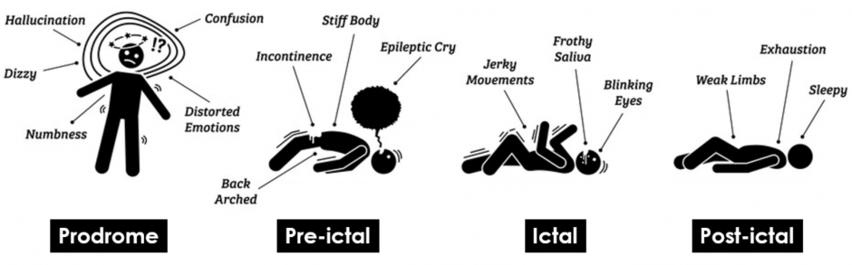
https://www.123rf.com/photo_107953001_stages-and-phases-of-a-seizure-illustrations-depicts-the-phases-when-a-person-get-a-seizure-which-ar.html
Research in predicting epileptic seizures predominantly revolves around predicting or detecting the pre-ictal stage so that the individual either receives some assistance or moves to a more secure environment for when they experience the ictal stage.
4. Related work and discussion
Several studies have proposed approaches designed to detect the pre-ictal with the help of electroencephalogram (EEG) patterns as these patterns may reflect the transition from the normal brain state (inter-ictal) to a state of hypersynchronous neuronal activity (ictal) (Engel et al 2008; Acharya et al 2013). The most commonly used dataset for pre-ictal and inter-ictal stage determination is the CHB-MIT Scalp EEG database, which was collected at the Children’s Hospital in Boston (Goldberger, A. et al 2000). This dataset consists of EEG recordings from paediatric subjects with intractable (drug-resistant) seizures. The subjects were monitored for up to several days following withdrawal of anti-seizure medication in order to characterise their seizures and assess their candidacy for surgical intervention. The medical time-series data was collected from 22 subjects (5 males, ages 3–22; and 17 females, ages 1.5–19). One advantage of this dataset is that it contains continuous long-term recordings that can last several hours combined with detailed clinical annotations about seizures times, which is a good source of ground-truth.
However, using EEG to determine the onset of a seizure poses two disadvantages. First, EEG caps are impractical for all-day use and are indiscreet. Second, there is some evidence of a racial bias in studies exhibiting the effectiveness of EEG caps in recording brain activity (Choy et al 2022). The authors state that EEG caps insufficiently capture data from participants with different hairstyles. Due to this, initial EEG studies excluded Black-American participants, resulting in less/no data from this demographic. This makes EEG-related advances less generalizable.
This warrants the need to look for alternate wearable technologies to detect/predict the pre-ictal stage. Other works have delved into the utilisation of electrocardiogram (ECG) data to detect pre-ictal behaviour. The justification for using ECG data comes from the fact that the onset of a seizure affects the autonomic nervous system of an individual. There are two types of autonomic nervous systems: sympathetic autonomic nervous system and parasympathetic autonomic nervous system. The primary function of the sympathetic autonomic nervous system is to stimulate the body’s fight-or-flight response. It does this by increasing the heart rate, dilating the bronchial tubules, dilating the pupil etc. It is this state that is triggered during the pre-ictal and ictal stages of a seizure. On the other hand, the parasympathetic autonomic nervous system restores the body to a state of calm by slowing the heart rate, constricting the bronchial tubules, constricting the pupils etc. Some works have associated a change in the autonomic nervous system to the onset of a seizure. These works have, hence, used heart rate features to monitor the seizure onset, stating that such features may be a good indicator of pre-ictal stage prediction (Lotufo et al 2012; Di Gennaro et al 2004; Hashimoto et al 2013).
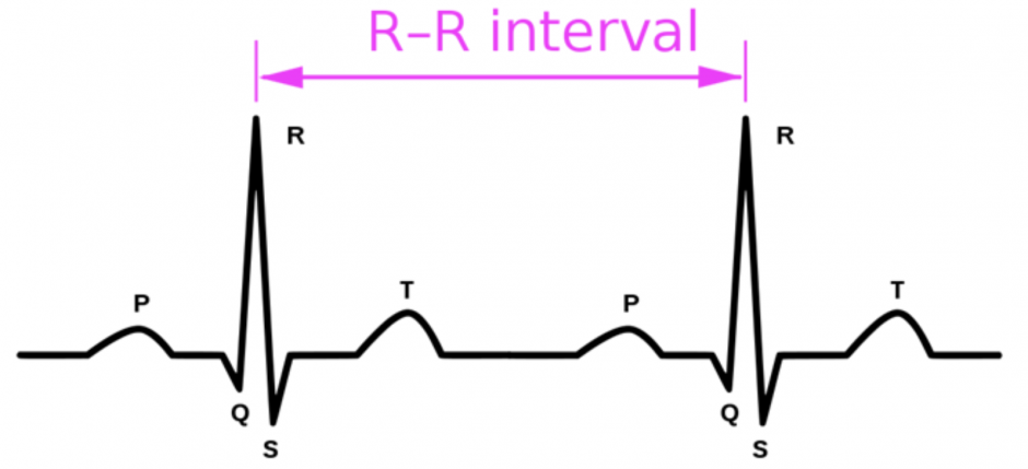
It must be noted that these extracted features are high-level data points and not the raw heart rate (HR) itself. This is because heart rate (HR) alone is unable to give information on the specific sympathetic and parasympathetic influences on heart rate control (Delamont et al 2011). A rapid increase in HR as is seen in a majority of tonic clonic seizures (i.e. seizures that involve both tonic/stiffening and clonic/twitching/jerking phases of muscle activity) can be due to either the withdrawal of cardiac parasympathetic activity or an increase in sympathetic activity or a combination of the two with the timing of the alterations impossible to determine purely from the HR data. Hence, instead of using HR, existing research using ECG data relies on mathematical features obtained from the R-R interval (see figure 2) (Akselrod et al 1981; Sleight et al 1995; Pagani et al 1986; Ghosh et al, 2017; Moridani et al, 2017; Yamakawa et al, 2020; Seifi et al, 2022). These mathematical features are of three kinds: time-domain, frequency-domain, and geometric. This work experiments with features from all 3 kinds as inputs to classical machine learning algorithms to observe feature importances.
5. Dataset
This solution is built on the dataset containing ECG and EEG signals (measured at a sampling rate of 512 Hz) acquired from 13 patients who have epilepsy (Billeci et al 2018). The dataset was collected from patients admitted to the Unit of Neurology and Neurophysiology, Department of Neurological and Neurosensorial Sciences, University of Siena, Italy. Each file in the dataset corresponds to one seizure episode and these files were stored in the EDF (European Data Format) format which is a standard file format designed for exchange and storage of medical time series data. For each file, there was an associated ground-truth text (TXT) file that included timestamps for experiment start/end and seizure start/end. We have also created a document that provides a low-level description of this dataset.
6. Data pre-processing
This is a binary classification task with 2 possible outputs for a given temporal ECG sample – pre-ictal and non pre-ictal. Hence, to train a model for a binary classification task, we need distinct temporal samples corresponding to either class. The following subsections explain the various pre-processing tasks that were performed on the raw ECG EDF files to make the resulting data appropriate for the binary classification task.
6.1. Extracting pre-ictal temporal data
To extract pre-ictal temporal samples from the ECG signals, we require timestamps corresponding to when the pre-ictal phase begins. As these pre-ictal timestamps were not provided in the ground-truth files, we had to estimate them. This is challenging as true pre-ictal durations may vary among individuals and even among seizure events experienced by the same individual (Bandarabadi et al 2015), and works that have been able to successfully differentiate between the two stages rely on EEG signals (e.g., Gadhoumi et al 2012). One work analysed the optimal pre-ictal period (OPP) from ninety-four seizure episodes (Bandarabadi et al 2015). The authors reported that the resulting OPPs ranged from 5 minutes up to 173 minutes, with an average value of 44.3 minutes. Given the limited sample size of our dataset (n=13), we decided to maximise the likelihood of understanding pre-ictal behaviour as well as the behaviour that occurs during its preceding stage. Hence, for our solution, we specified 40 minutes as the OPP preceding a seizure episode, which helps us identify pre-ictal datapoints.
We extract non pre-ictal data points in two different ways corresponding to two different scenarios (see figures 3 and 4). When the pre-ictal phase begins 40 minutes after the experiment starts, temporal samples from the beginning of the experiment to the beginning of the pre-ictal phase along with those from the end of the seizure to the end of the experiment are extracted as non pre-ictal datapoints (figure 3). Alternatively, when the pre-ictal phase begins within 40 minutes of the experiment starting, only the temporal samples from the end of the seizure to the end of the experiment are extracted as non pre-ictal datapoints (figure 4).
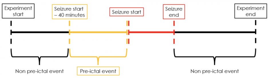
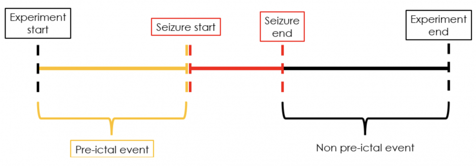
Figure 3: Extracting pre-ictal and non pre-ictal temporal samples when pre-ictal phase begins 40 minutes after experiment starts
Figure 4: Extracting pre-ictal and non pre-ictal temporal samples when pre-ictal phase begins within 40 minutes of the experiment starting
6.2. Splitting the temporal samples
Although pre-ictal symptoms worsen and are, hence, more pronounced when the individual is close to experiencing the seizure (Mula et al 2013), we chose to regard the entire 40-minute sequential data with equal importance. This was done to ensure that the model can detect the pre-ictal phase even when the symptoms are relatively less pronounced. We then split these 40 minute temporal samples into 5 minute samples so that the solution model can make predictions on 5 minute heart rate variations. This is because past work has identified 5 minutes as the minimum optimal duration for HRV feature extraction [Catai et al 2020; Sheridan et al 2021; Circulation article 1996].
6.3. Denoising and R-peaks determination
We follow the same pre-processing steps as in Billeci et al (2018). ECG signals were first analysed for impulsive artefacts removal, power-line interference cancelling (50Hz), baseline wandering removal, signal-to-noise ratio improvement. Impulsive artefacts cancelling was obtained by computing the absolute difference between the original signal and the signal obtained by median filtering (60 ms window). Then if the absolute difference of a specific segment of signal exceeded a threshold (estimated considering the maximum of this difference) that segment was considered as an artefact and its values were assigned with the average of the values of the original signal immediately before and after the segment. Baseline wandering removal was obtained by applying a low-pass first order Butterworth filter in forward and backward directions (total cutoff frequency at 3.1 Hz) and subtracting the signal obtained from the original signal. The occurrence of residual artefacts, due to the filter delay in tracking fast baseline movements, was then verified. If the amplitude and the duration of residual artefacts exceed certain thresholds, a median filtering (0.26 s window) was applied.After these steps, the signal was interpolated to 1024 KHz to get a precise time location and the QRS complexes were detected to reconstruct the RR series.
7. Solution
Following the preprocessing steps in subsections 6.1-6.3, we were able to generate 72 data samples (26 pre-ictal samples and 46 non pre-ictal samples). As the classes were highly imbalanced, we used Synthetic Minority Oversampling (SMOTE) [Chawla et al, 2002] to generate synthetic samples for the minority class (i.e. pre-ictal samples). SMOTE is an algorithm that performs data augmentation by creating synthetic data points based on the original data points and its advantage is that you are not generating duplicates, but rather creating synthetic data points that are slightly different from the original data points. Using SMOTE resulted in having 92 data samples (46 pre-ictal and 46 non pre-ictal). From these samples, we extracted 24 features. These features are classified into time domain (16), frequency domain (7), and geometric (1). Tables 1-3 list out the features and their definitions.
Table 1: Extracted time domain features from the RR-series temporal samples
| Time domain features | Definition |
| Mean nni | The mean of RR-intervals |
| Sdnn | The standard deviation of the time interval between RR-intervals |
| Sdsd | The standard deviation of differences between adjacent RR-intervals |
| Nni 50 | Number of interval differences of successive RR-intervals greater than 50 ms |
| Pnni 50 | The proportion derived by dividing nni_50 by the total number of RR-intervals |
| Nni 20 | Number of interval differences of successive RR-intervals greater than 20 ms |
| Pnni 20 | The proportion derived by dividing nni_20 by the total number of RR-intervals |
| Rmssd | The square root of the mean of the sum of the squares of differences between adjacent NN-intervals |
| Median nni | Median Absolute values of the successive differences between the RR-intervals |
| Range nni | Median Absolute values of the successive differences between the RR-intervals |
| Cvsd | rmssd divided by mean_nni |
| Cvnni | Coefficient of variation equal to the ratio of sdnn divided by mean_nni |
| Mean HR | Mean heart rate |
| Max HR | Max heart rate |
| Min HR | Min heart rate |
| Std HR | Standard deviation of heart rate |
Table 2: Extracted frequency domain features from the RR-series temporal samples
| Frequency domain features | Definition |
| Lf | HRV variance in Low Frequency |
| Hf | HRV variance in High Frequency |
| Lf Hf ratio | HRV variance in Low Frequency/HRV variance in High Frequency |
| Lfnu | Normalized Lf power |
| Hfnu | Normalized Hf power |
| Total power | Total power density spectral |
| Vlf | HRV variance in Very Low Frequency: Reflect an intrinsic rhythm produced by the heart which is modulated primarily by sympathetic activity |
Table 3: Extracted geometrical features from the RR-series temporal samples
| Geometrical features | Definition |
| Triangular Index | Integral of the number of all NN-intervals / maximum of the density distribution |
Based on the limited dataset size (n=92) despite oversampling, we resorted to applying classical machine learning models for sample classification. As we only had data from13 patients, we wanted to use as much of the data as possible for training, hence, as a proof-of-concept solution, we randomly split the 92 samples into train, validation and test sets to determine the most optimal predictive model. Sample-level split (as opposed to participant-level split) is also underpinned by the fact that even for the same individual, pre-ictal and non pre-ictal behaviour may vary across seizure episodes [Gadhoumi et al 2012].
8. Results and discussion
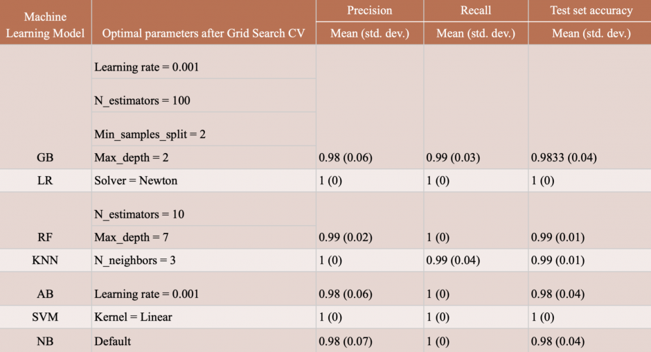
The classical machine learning models we chose were Gradient Boosting (GB), Adaptive Boosting (AB), Logistic Regression (LR), Naive Bayes (NB), K Nearest Neighbours (KNN), Random Forest (RF), and Support Vector Machine (SVM). We used 85% (n=78) of the data for nested cross validation and held 15% (n=14) of it to determine final test performance on data that the model has never encountered before. For all models, we performed a Grid Search CV for hyper-parameter tuning and for each parameter configuration, we performed 10 iterations of 10-fold cross validation to assess the performance of the model on the entirety of the 85% dataset. For performance measure, we used the metrics of precision (out of all events that were classified as pre-ictal, how many were really pre-ictal?), recall (out of all truly preictal events, how many were classified as preictal?), and accuracy (overall, how well did the classifier do?). Table 4 presents the best results obtained. As can be observed, all models have a near perfect performance when distinguishing between ictal and pre-ictal samples. While this is an encouraging result, it also implies that the dataset size, despite the minority class oversampling, is insufficient for a more sophisticated classifier which might be able to model more intricate characteristics of a pre-ictal or non pre-ictal sample.
Table 4: Results of the machine learning models along with their best performing hyperparameter configurations and corresponding accuracy scores.
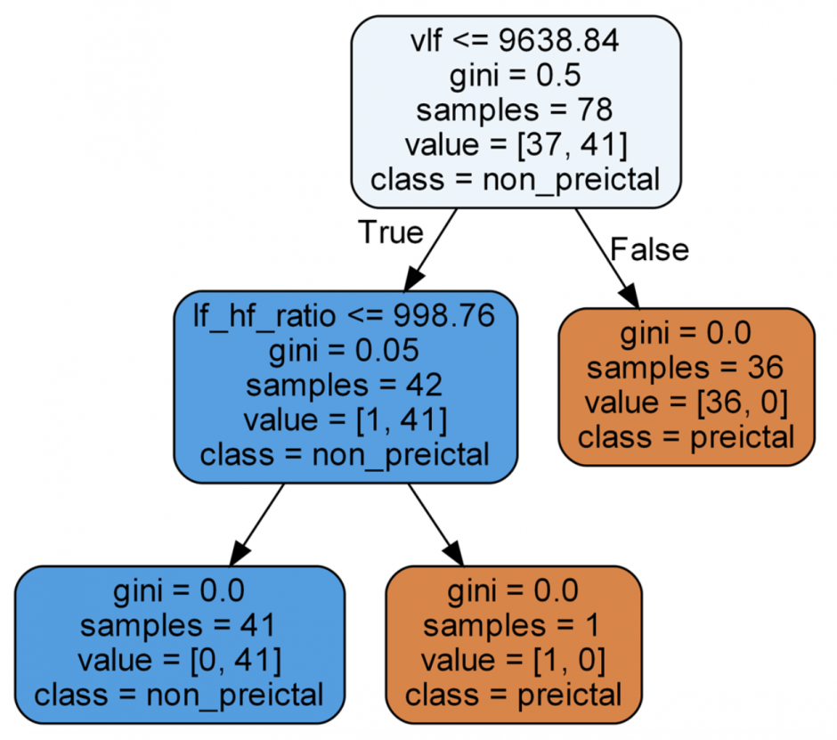
Another benefit of using classical machine learning models is their inherent interpretability. This can help us understand what data features were considered most predictive for the task. For instance, for a trained random forest model, the best performing decision tree can be extracted and its decision-making pathway can be generated to see what features are considered most indicative. Figure 5 shows how the decision tree uses specific data features to make its predictions. “Gini” in the nodes refers to the Gini Index, which is a powerful measure of the randomness/ impurity/entropy in the values of a dataset. Gini Index aims to decrease the impurities from the root nodes (at the top of decision tree) to the leaf nodes (vertical branches down the decision tree) of a decision tree model. Hence, from an interpretability perspective, this feature of classical machine learning models can potentially be used to provide explanations for the model’s predictions. This can be especially useful in cases when the user wants to know why the model thinks the user will have a seizure soon.
9. Conclusion and future work
This work explores a range of simple machine learning solutions for distinguishing between pre-ictal and non pre-ictal samples using 5 minute heart rate temporal data. This work deals with how raw ECG data can be pre-processed to extract R-R intervals for calculating a myriad of heart rate variability (HRV) features and how the data can be artificially balanced with synthetic minority class oversampling techniques. While the solution models have a near perfect performance in this classification task, it must be noted that a more realistic solution would involve designing a classifier for each patient which is attuned to their personal pre-ictal behavioural characteristics. However, this would require a large dataset for each patient, which may involve months of data collection. Future approaches should first focus on collecting data whose size is much larger that the one presented here and also include naturally occurring non pre-ictal samples. This is because the non pre-ictal samples extracted from this dataset were from all sequential data points which are not a part of the pre-ictal phase. It is possible that the effects of pre-ictal and ictal phases last longer than the durations assumed here, so having information on long periods of time with no ictal phase would be useful. Lastly, future approaches should explore extracting pre-ictal samples without a predefined cutoff as the number varies among patients and even among seizure episodes for the same patient. Possible paths may involve unsupervised learning techniques such as clustering [Leal et al, 2021].
10. References
Click for more details
[Viscidi et al 2013] Viscidi EW, Triche EW, Pescosolido MF, McLean RL, Joseph RM, Spence SJ, Morrow EM. Clinical characteristics of children with autism spectrum disorder and co-occurring epilepsy. PLoS One. 2013 Jul 4;8(7):e67797. doi: 10.1371/journal.pone.0067797. PMID: 23861807; PMCID: PMC3701630.
[Ewen et al 2019] Ewen JB, Marvin AR, Law K, Lipkin PH. Epilepsy and Autism Severity: A Study of 6,975 Children. Autism Res. 2019 Aug;12(8):1251-1259. doi: 10.1002/aur.2132. Epub 2019 May 24. PMID: 31124277.
[Achkar et al 2015] El Achkar CM, Spence SJ. Clinical characteristics of children and young adults with co-occurring autism spectrum disorder and epilepsy. Epilepsy Behav. 2015 Jun;47:183-90. doi: 10.1016/j.yebeh.2014.12.022. Epub 2015 Jan 15. PMID: 25599987.
[Novarino et al 2013] Novarino, G., Baek, S. T., & Gleeson, J. G. (2013). The sacred disease: the puzzling genetics of epileptic disorders. Neuron, 80(1), 9–11. https://doi.org/10.1016/j.neuron.2013.09.019
[Frank et al 2021] Frank, Yitzchak. “The Neurological Manifestations of Phelan-McDermid Syndrome.” Pediatric Neurology 122 (2021): 59-64.
[Borlot et al 2019] Borlot, Felippe, Bruno Ivo de Almeida, Shari L. Combe, Danielle M. Andrade, Francis M. Filloux, and Kenneth A. Myers. “Clinical utility of multigene panel testing in adults with epilepsy and intellectual disability.” Epilepsia 60, no. 8 (2019): 1661-1669.
[Engel et al 2008] Engel, J., Dichter, M. A. & Schwartzkroin, P. A. Basic Mechanisms of Human Epilepsy. In Engel, J. & Pedley, T. A. (eds.) Epilepsy: a comprehensive textbook, chap. 41, 495–508 (Wolters Kluwer Health/Lippincott Williams & Wilkins, 2008), 2nd edition.
[Acharya et al 2013] Acharya, U. R., Vinitha Sree, S., Swapna, G., Martis, R. J. & Suri, J. S. Automated EEG analysis of epilepsy: a review. KnowledgeBased Syst. 45, 147–165. https://doi.org/10.1016/j.knosys.2013.02.014 (2013).
[Goldberger, A. et al 2000] Goldberger, A., L. Amaral, L. Glass, J. Hausdorff, P. C. Ivanov, R. Mark, J. E. Mietus, G. B. Moody, C. K. Peng, and H. E. Stanley. “PhysioBank, PhysioToolkit, and PhysioNet: Components of a new research resource for complex physiologic signals. Circulation [Online]. 101 (23), pp. e215–e220.” (2000).
[Choy et al 2022] Choy, Tricia, Elizabeth Baker, and Katherine Stavropoulos. “Systemic racism in EEG Research: considerations and potential solutions.” Affective Science 3, no. 1 (2022): 14-20.
[Delamont et al 2011] Delamont, Robert S., and Matthew C. Walker. “Pre-ictal autonomic changes.” Epilepsy research 97, no. 3 (2011): 267-272.
[Goldberger et al 2017] Goldberger, Ary L., Zachary D. Goldberger, and Alexei Shvilkin. Clinical electrocardiography: a simplified approach e-book. Elsevier Health Sciences, 2017.
[Akselrod et al 1981] Akselrod, Solange, David Gordon, F. Andrew Ubel, Daniel C. Shannon, A. Clifford Berger, and Richard J. Cohen. “Power spectrum analysis of heart rate fluctuation: a quantitative probe of beat-to-beat cardiovascular control.” science 213, no. 4504 (1981): 220-222.
[Sleight et al 1995] Sleight, Peter, Maria Teresa La Rovere, Andrea Mortara, Gianni Pinna, Roberto Maestri, Stefano Leuzzi, Beatrice Bianchini, Luigi Tavazzi, and Luciano Bernardi. “Physiology and pathophysiology of heart rate and blood pressure variability in humans: is power spectral analysis largely an index of baroreflex gain?.” Clinical science 88, no. 1 (1995): 103-109.
[Pagani et al 1986] Pagani, Massimo, Federico Lombardi, Stefano Guzzetti, Ornella Rimoldi, Raffaello Furlan, Paolo Pizzinelli, Giulia Sandrone, Gabriella Malfatto, Simonetta Dell’Orto, and Emanuela Piccaluga. “Power spectral analysis of heart rate and arterial pressure variabilities as a marker of sympatho-vagal interaction in man and conscious dog.” Circulation research 59, no. 2 (1986): 178-193.
[Lotufo et al 2012] Lotufo, Paulo A., Leandro Valiengo, Isabela M. Bensenor, and Andre R. Brunoni. “A systematic review and meta‐analysis of heart rate variability in epilepsy and antiepileptic drugs.” Epilepsia 53, no. 2 (2012): 272-282.
[Di Gennaro et a, 2004] Di Gennaro, Giancarlo, Pier Paolo Quarato, Fabio Sebastiano, Vincenzo Esposito, Paolo Onorati, Liliana G. Grammaldo, Giulio N. Meldolesi et al. “Ictal heart rate increase precedes EEG discharge in drug-resistant mesial temporal lobe seizures.” Clinical neurophysiology 115, no. 5 (2004): 1169-1177.
[Hashimoto et al 2013] Hashimoto, Hirotsugu, Koichi Fujiwara, Yoko Suzuki, Miho Miyajima, Toshitaka Yamakawa, Manabu Kano, Taketoshi Maehara et al. “Heart rate variability features for epilepsy seizure prediction.” In 2013 Asia-Pacific Signal and Information Processing Association Annual Summit and Conference, pp. 1-4. IEEE, 2013.
[Ghosh et al 2017] Ghosh, Arijit, Anasua Sarkar, Tarak Das, and Piyali Basak. “Pre-ictal epileptic seizure prediction based on ECG signal analysis.” In 2017 2nd International Conference for Convergence in Technology (I2CT), pp. 920-925. IEEE, 2017.
[Moridani et al 2017] Moridani, M., and H. Farhadi. “Heart rate variability as a biomarker for epilepsy seizure prediction.” Clin. Study 3, no. 8 (2017): 3-8.
[Yamakawa et al 2020] Yamakawa, Toshitaka, Miho Miyajima, Koichi Fujiwara, Manabu Kano, Yoko Suzuki, Yutaka Watanabe, Satsuki Watanabe, Tohru Hoshida, Motoki Inaji, and Taketoshi Maehara. “Wearable epileptic seizure prediction system with machine-learning-based anomaly detection of heart rate variability.” Sensors 20, no. 14 (2020): 3987.
[Seifi et al 2022] Seifi, Bahare, Mahsa Barfi, and Mansour Esmaeilpour. “ECG-Based Prediction of Epileptic Seizures Using Machine Learning Methods.” In 2022 9th Iranian Joint Congress on Fuzzy and Intelligent Systems (CFIS), pp. 1-7. IEEE, 2022.
[Billeci et al 2018] Billeci, Lucia, Daniela Marino, Laura Insana, Giampaolo Vatti, and Maurizio Varanini. “Patient-specific seizure prediction based on heart rate variability and recurrence quantification analysis.” PloS one 13, no. 9 (2018): e0204339.
[Gadhoumi et al 2012] Gadhoumi, Kais, Jean-Marc Lina, and Jean Gotman. “Discriminating preictal and interictal states in patients with temporal lobe epilepsy using wavelet analysis of intracerebral EEG.” Clinical neurophysiology 123, no. 10 (2012): 1906-1916.
[Bandarabadi et al 2015] Bandarabadi, Mojtaba, Jalil Rasekhi, César A. Teixeira, Mohammad R. Karami, and António Dourado. “On the proper selection of preictal period for seizure prediction.” Epilepsy & Behavior 46 (2015): 158-166.
[Mula et al 2013] Mula, M. “Pre-ictal psychiatric symptoms.” Epilepsy & Behavior 28, no. 2 (2013): 318.
[Fattorusso et al 2021] Fattorusso, Antonella, Sara Matricardi, Elisabetta Mencaroni, Giovanni Battista Dell’Isola, Giuseppe Di Cara, Pasquale Striano, and Alberto Verrotti. “The Pharmacoresistant Epilepsy: an overview on existant and new emerging therapies.” Frontiers in Neurology 12 (2021): 1030.
[Circulation article 1996] Electrophysiology, Task Force of the European Society of Cardiology, the North American Society of Pacing. “Heart rate variability: standards of measurement, physiological interpretation, and clinical use.” Circulation 93, no. 5 (1996): 1043-1065.
[Catai et al 2020] Catai, Aparecida Maria, Carlos Marcelo Pastre, Moacir Fernades de Godoy, Ester da Silva, Anielle Christine de Medeiros Takahashi, and Luiz Carlos Marques Vanderlei. “Heart rate variability: are you using it properly? Standardisation checklist of procedures.” Brazilian journal of physical therapy 24, no. 2 (2020): 91-102.
[Sheridan et al 2021] Sheridan, David C., Karyssa N. Domingo, Ryan Dehart, and Steven D. Baker. “Heart Rate Variability Duration: Expanding the Ability of Wearable Technology to Improve Outpatient Monitoring?.” Frontiers in Psychiatry 12 (2021): 943.
[Chawla et al, 2002] Chawla, Nitesh V., Kevin W. Bowyer, Lawrence O. Hall, and W. Philip Kegelmeyer. “SMOTE: synthetic minority over-sampling technique.” Journal of artificial intelligence research 16 (2002): 321-357.
[Leal et al, 2021] Leal, Adriana, Mauro F. Pinto, Fábio Lopes, Anna M. Bianchi, Jorge Henriques, Maria G. Ruano, Paulo de Carvalho, António Dourado, and César A. Teixeira. “Heart rate variability analysis for the identification of the preictal interval in patients with drug-resistant epilepsy.” Scientific reports 11, no. 1 (2021): 1-11.